
Why High-Scale Systems Need Better Data Layer Decisions

Data layers rarely fail because they cannot hold the data. They fail because they waste effort fetching data that is not there, recomputing answers they already had, or letting one workload starve another. A product page makes ten round trips for content that has not changed all day. A join multiplies a single order into hundreds of rows during a sale. A reporting query locks the table that processes payments. None of these are surprises. They are the predictable consequences of design choices made before the load arrived.
The difference between data layers that scale and data layers that stall is rarely the storage engine on the box. It is whether the team understood a handful of foundational patterns and applied them with intent before traffic forced the issue.
Executive Summary: Core Database and Storage Patterns for High-Scale Systems
- Bloom Filters in Databases. Cheap memory checks beat expensive disk seeks. A small probabilistic guard in front of every read eliminates negative lookups before they reach the storage layer.
- Database Joins from First Principles. A join is a data movement and comparison problem, not a syntax convenience. The cost compounds with data growth, it does not add to it.
- Caching Strategies in Databases. Most data is read far more often than it is written. Treating that imbalance with intent is the difference between graceful scale and a campaign-day incident.
- OLTP vs OLAP Workloads. One workload records what happens. The other explains it. Asking a single engine to do both is how cascading slowdowns begin.
- Event Sourcing as a Persistence Model. Storing only the current state throws away history. For domains where the journey matters as much as the destination, the journey is what gets persisted.
1. Bloom Filters in Databases: A Cheap Memory Check in Front of Expensive Reads
Read paths dominate modern data systems. Cache lookups, secondary index probes, SSTable scans inside an LSM tree, distributed shard queries. A surprising proportion of those reads are for keys that simply do not exist. Without a guard in front, every negative lookup pays the full cost of a disk seek or a network round trip. Multiply that across millions of queries a day and you get inflated tail latency, wasted I/O, and cloud bills that grow faster than the business.
A bloom filter is a fixed-size bit array paired with several independent hash functions. Inserts hash a key multiple times and set the corresponding bits. Lookups hash the same way and check whether all those bits are set. If any bit is unset, the key is guaranteed absent. If all bits are set, the key is probably present, but not certainly. Bloom filters trade certainty in one direction (false positives) for an absolute guarantee in the other (no false negatives).
The design parameters are explicit and tunable. For an expected cardinality n and a target false-positive rate p, the optimal bit-array size is m ≈ -n ln(p) / (ln 2)² and the optimal number of hash functions is k ≈ (m/n) ln 2. Memory cost is not something the system imposes on you. It is something you choose.
Where a bloom filter earns its keep in a real system:
- In front of SSTable lookups in an LSM-tree, so negative lookups skip disk entirely
- In front of distributed shard queries, so the coordinator does not fan out for a key that exists nowhere on the cluster
- In front of expensive cache loads, so misses for non-existent items do not pile on to the primary database
- In stream processing, to deduplicate against a large set of seen IDs without storing them in full
When teams skipped it: An LSM-backed key-value store began showing P99 read latency climbing into multi-second territory under peak load. The reflexive call was to add nodes. The actual culprit was a configuration choice made months earlier to disable bloom filters and save memory. Negative lookups for non-existent user IDs were touching SSTables at every level on every miss. Re-enabling the filters, at a memory cost smaller than a single application pod, collapsed disk reads and stabilised tail latency without a new machine. The cost of skipping a few megabytes of bit array was a three-week incident.
Performance work is often misframed as making things faster. A great deal of it is making things avoidable. Bloom filters are the cleanest example: cheap, mathematically bounded, and ruthlessly effective at ruling out work that did not need to happen.

2. Database Joins from First Principles: The Real Cost Behind the Syntax
Most production database incidents do not start with exotic bugs. They start with a feature shipping, data growing, and one join that worked beautifully in staging. Joins are among the most powerful tools in a relational engine. They are also among the most expensive operations when written without understanding what they actually do.
A join is not a SQL keyword. It is a data movement and comparison operation that produces a new result set from rows of two or more inputs that share a relationship. Everything from INNER JOIN and LEFT JOIN to hash join, merge join, and nested loop join is an optimisation around that single idea.
Every join carries three costs:
- Matching cost: comparing join keys across inputs
- Access cost: reading rows from disk, memory, or the network
- Cardinality cost: producing more rows than the inputs, sometimes by orders of magnitude
The strategy the planner picks depends on the data shape:
- Nested loop join compares row by row. Cheap for small inputs, brutal for large ones.
- Hash join builds an in-memory hash table on the smaller side and probes it. Fast, but memory-bound and sensitive to skew.
- Merge join requires sorted inputs and walks them in lockstep. Efficient when the sort cost has already been paid by an index.
- Indexes reduce access cost. They do not eliminate matching or cardinality cost.
The non-obvious truth is that join cost does not scale linearly with data. A join that produces a million-row intermediate result on a hundred-thousand-row input is not slow. It is misdesigned.
When teams didn't follow this: A team built an Order Overview API that joined orders, order items, shipments, and payments in a single query. It performed well in staging, where each order had one shipment and one payment. A festive sale changed the assumptions. Orders gained partial shipments and split payments. A single logical order became hundreds of result rows. Pagination broke. Database CPU saturated. The fix was not query tuning. It was redesign. The team split the reads, pre-aggregated shipment and payment summaries on to the order row, and pulled detailed lines via separate endpoints. Runtime joins on the hot path were removed entirely.
Joins encode assumptions about cardinality and growth that are easy to make at design time and expensive to remediate at scale. Teams that understand the underlying cost model build schemas, queries, and APIs that survive the next traffic spike. Teams that do not, redesign under pressure.
3. Caching Strategies in Databases: The Difference Between Surviving a Campaign and Pausing It
Every successful system eventually meets the same wall. The database becomes the bottleneck. The engine on the other side rarely matters: most workloads read the same data thousands of times more often than they write it. Product details, user profiles, configuration, pricing rules, feature flags. None of it changes between requests. Asking the primary database for the same answer every time is, at scale, a self-inflicted cost.
Caching moves frequently read data into a faster layer that sits between the application and the system of record. The mechanics differ by strategy, but the intent is consistent: serve the common case from memory, send only the uncommon case to durable storage.
The four production caching patterns worth knowing in depth:
- Cache-aside (lazy loading). The application checks the cache first. On a miss, it reads from the database and populates the cache. Simple, robust, and the default for most read-heavy workloads. The drawback is a cold-start penalty on each new key and the risk of a stampede when a hot key expires.
- Read-through. The cache layer itself fetches from the database on a miss. Application code is simpler at the cost of tighter coupling to the cache layer.
- Write-through. Writes go to the cache first and synchronously through to the database. Cache and store stay consistent at the cost of higher write latency.
- Write-behind (write-back). Writes go to the cache immediately and are flushed to the database asynchronously. Writes are fast, but data loss is real if the cache fails before the flush completes.
Beyond these, time-to-live (TTL) policies, eviction strategies (LRU, LFU, ARC), and cache key design decide whether the cache stays effective under load. Production systems typically combine several patterns: cache-aside for the product catalogue, write-through for inventory, TTL for pricing, and explicit invalidation for anything that must reflect a change immediately.
Two failure modes deserve named attention because they catch teams by surprise:
- Cache stampede. A popular key expires and a thousand concurrent requests miss at the same instant, each triggering a database read for the same value. Mitigations include request coalescing, probabilistic early expiration, and lock-based refresh.
- Hot keys. A small number of keys concentrate disproportionate traffic on a single cache node. Per-key replication or sharding strategies spread the load.
When teams didn't follow this: A retail platform prepared for a festive sale expecting five times normal traffic. The product catalogue service queried the database directly on every request. Within minutes of launch, database CPU hit one hundred percent. Queries slowed. Timeouts cascaded into unrelated services sharing the same database. The data being fetched, product descriptions and images, had not changed all day. A cache-aside layer with a few minutes of TTL would have absorbed more than ninety percent of the load. Instead the campaign was paused mid-flight while caching was rolled out under duress.
Caching is not a performance trick. It is the load model your data layer needs to survive a real spike. Systems that treat the database as an infinite resource eventually meet its actual limits at the worst possible moment.
4. OLTP vs OLAP Workloads: Why One Database Rarely Serves Both Well
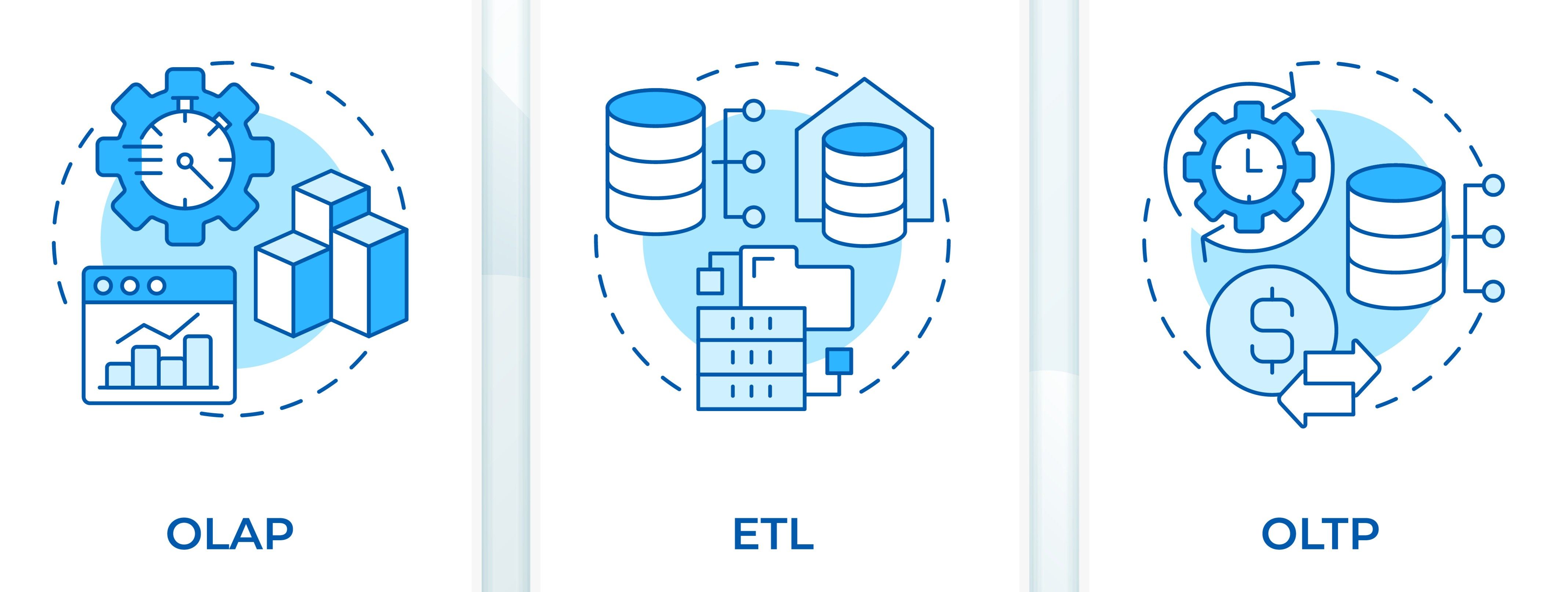
Some systems record what happens. Others explain it. The first set processes orders, payments, and updates as they occur, holding the system of record for the business. The second scans across months or years of those records to find patterns: revenue trends, churn signals, fraud rings, demand forecasts. These are two workloads with two cost profiles. Asking one engine to handle both is among the most common, and most expensive, architectural shortcuts a team can take.
OLTP (Online Transaction Processing) workloads are short, concurrent, and write-heavy or mixed. Each transaction touches a small number of rows, runs in milliseconds, and demands strict consistency. Schemas are typically normalised to preserve integrity and reduce duplication. The engineering priorities are low latency, high concurrency, and transactional isolation.
OLAP (Online Analytical Processing) workloads are long, read-heavy, and aggregation-driven. A single query may scan billions of rows across multiple dimensions. Latency in seconds, sometimes minutes, is acceptable. Schemas are denormalised, modelled as star or snowflake patterns, and physically optimised for sequential scans, column compression, and partition pruning. The engineering priorities are throughput, scan efficiency, and parallel execution.
| Dimension | OLTP | OLAP |
|---|---|---|
| Query shape | Short, point lookups, narrow updates | Long, wide scans, aggregations |
| Rows per query | A few to a few hundred | Millions to billions |
| Schema | Normalised | Denormalised, star or snowflake |
| Storage layout | Row-store | Often columnar |
| Concurrency | Very high, many users | Lower, fewer concurrent queries |
| Latency target | Milliseconds | Seconds to minutes |
| Business role | Runs operations | Informs decisions |
The two profiles stress storage engines in opposite directions. OLTP wants short row-level operations, narrow indexes, and tight isolation. OLAP wants wide scans, columnar layouts, and aggregation pushdown. A row-store engine tuned for transactions has neither the storage format nor the query planner to run analytical queries well at scale. A columnar engine tuned for analytics struggles with single-row updates and concurrent transactions.
The architectural pattern that consistently works:
- An operational store for live application traffic, sized and tuned for transactional load
- A replicated path to an analytical store via change data capture or batch extract
- A warehouse, lakehouse, or columnar engine for reporting, dashboards, and exploratory analysis
- A clear policy on which workloads can ever touch the operational store directly
Hybrid transactional and analytical processing (HTAP) engines exist and have their place, but they remain specialised. For most enterprises, physical separation is cheaper and more predictable than convergence on a single engine.
When teams didn't follow this: A product team built a customer dashboard directly on the primary operational database. It worked at first, when filters were limited and date ranges short. Then leadership asked for longer time ranges, more filters, and near-real-time charts. Analytical queries began scanning large tables while the same database processed live checkouts. API latency climbed. Deadlocks became routine during peak traffic. A read replica helped briefly, then ran into the same scan problems. The durable fix was structural: change data capture into a columnar analytical store, with the dashboard rebuilt against that store. The original incident was diagnosed as a query tuning problem. It was actually an architectural one.
Strong data architectures separate workloads by their nature, not by their owner. One database keeps the business running. Another helps the business think. Confusing the two is a recurring source of avoidable incidents.
5. Event Sourcing as a Persistence Model: When the Journey Matters as Much as the Destination
Most applications persist the current state of an entity. The user's balance is one figure. The order's status is one value. The ticket is open or closed. This model is efficient and serves the majority of CRUD systems well. It also throws away history every time it overwrites a row. For domains where auditability, reconstruction, and business causality matter, that history is the actual asset.
Event sourcing stores every meaningful change as an immutable event in an append-only log. The current state is not the source of truth. The event stream is. Current state is derived by replaying events in order. A bank account is not stored as a balance. It is stored as AccountOpened, DepositMade, WithdrawalMade, TransferReceived, FeeApplied. The balance is a function of the sequence.
The benefits, when the domain fits:
- A complete audit trail by construction, not by retrofit
- Time-travel queries that reconstruct state as of any historical moment
- Multiple projections from the same event stream, each tailored for a different read use case
- A natural integration model, since downstream services subscribe to events that have already happened
- Preserved domain language, because events express business intent (
PaymentCaptured,RefundInitiated) rather than row-level mutations
The pattern almost always travels with CQRS (Command Query Responsibility Segregation). The write path appends events to the event store. The read path serves queries from projections built by processing those events. The two sides scale independently and can use different storage technologies.
Event sourcing introduces costs any team adopting it must plan for:
- Schema evolution is hard because events live forever. Adding a field is easy. Renaming or restructuring requires deliberate versioning strategies.
- Replay performance matters because rebuilding a projection from a billion events is not instant. Snapshots reduce replay cost but introduce their own complexity.
- Eventual consistency between the event store and projections is intrinsic to the model, not a defect to engineer around.
- Idempotency in event handlers is non-negotiable, because at-least-once delivery is the realistic default.
When teams didn't follow this: A payments platform stored only the current transaction status. A customer disputed a charge, claiming a debit, a refund, and a second debit had all occurred. The database showed settled. Logs were scattered across three services, with retention already expired in one of them. Reconstructing the actual sequence required pulling gateway callbacks, retry job traces, and reconciliation files across multiple teams over several days. Had the platform stored events such as PaymentInitiated, GatewayTimeoutReceived, RetryScheduled, RefundProcessed, and SettlementCompleted, the timeline would have been a single ordered query. The dispute was eventually resolved. The engineering cost of reconstructing history that was never recorded was the actual lesson.
Event sourcing is not a default. It is a deliberate choice for domains where the path to the current state is itself information the business needs. Applied to a simple CRUD system, it adds complexity that returns no value. Applied to a payments ledger, an order management platform, or a regulated workflow, it pays back in clarity, auditability, and integration reach.
The Common Thread: Data Layers Are Designed for Their Workload, Not Inherited By Default
These five patterns reinforce each other in ways that show up at scale. Bloom filters reduce wasted reads at the storage layer. Joins designed from first principles reduce wasted work at the query layer. Caching reduces load on whichever tier is most expensive to scale. Workload separation makes sure each engine is solving the problem it was built for. Event sourcing makes sure the history of change is recoverable when the business actually needs it.
The pattern running through all of them is intentionality: deciding what the data layer should do under load, rather than discovering it under outage. Pick one section. Trace it through the most painful data path in your system this week. The cost of acting on these patterns early is always smaller than the cost of acting on them under pressure.
Databases and Storage Patterns FAQ
1. What is a bloom filter and where is it most useful in a database? A bloom filter is a small probabilistic data structure that answers "is this key definitely absent?" very quickly and at low memory cost. It is most useful in front of expensive read paths, including LSM-tree SSTable lookups, distributed shard queries, and cache loads, where a negative lookup would otherwise pay the full cost of disk or network access. The tunable false-positive rate lets engineers choose the memory-versus-I/O trade-off explicitly.
2. Why do joins that work in staging fail in production? Staging data rarely reflects production cardinality. A join that produces one row per order in staging may produce hundreds per order in production once partial shipments or split payments enter the mix. Join cost compounds with data growth rather than adding to it, which is why a query that performs well at small scale can collapse abruptly once real data shape arrives.
3. Which caching strategy should we start with? Cache-aside is the default for most read-heavy workloads because it is simple, robust, and caches only what is actually requested. Add write-through, write-behind, or explicit invalidation when freshness matters more than write latency or when consistency between the cache and the database has to be tight. Plan for cache stampede and hot key problems before they happen, not after.
4. When should we separate OLTP and OLAP workloads? Earlier than feels necessary. The signal is not a specific traffic threshold; it is the moment analytical queries begin appearing on the same engine that serves live transactions. Read replicas can buy time. Change data capture into a columnar warehouse or lakehouse is the durable fix, and it is far cheaper to set up before an incident than after one.
5. Is event sourcing worth the complexity for a typical application? For a typical CRUD application, no. Event sourcing adds schema evolution, projection rebuild, and eventual consistency concerns that a state-storing model avoids. It pays back when audit, reconstruction, time-travel queries, or complex domain integration are first-order requirements, which is common in payments, ledgers, order management, and regulated workflows.
Learn more about Tarento's Data & Analytics Services | DataVolve: A Modern Data Platform for Enterprise Scale


Snowflake vs Databricks: Choosing the Right Enterprise Data Platform in 2026